Custom Dynamic Window Approach Implementation for Nav

Introduction to DWA Planner

Overview

This project implements a custom Dynamic Window Approach (DWA) local planner for ROS 2 Humble and demonstrates it on TurtleBot3 in Gazebo. The implementation is compact and pragmatic: it samples feasible (linear, angular) velocity pairs inside a dynamic window, simulates short-rollout trajectories, scores each rollout with a small cost function, and executes the velocity pair with the lowest cost. The code and launch instructions are in the repository linked above.

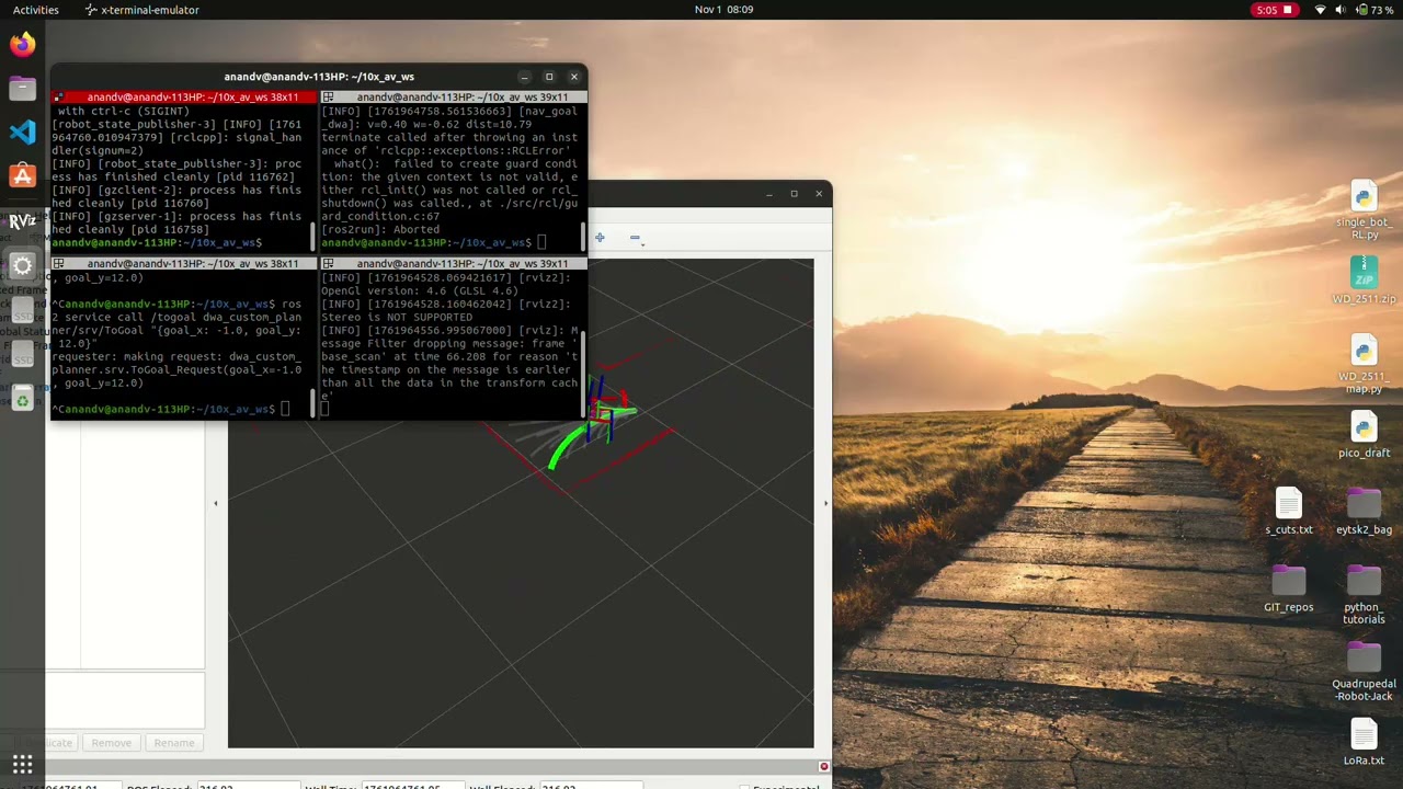
*Figure 1 — Sampled rollouts (grey) and the selected trajectory (bright). Frame from demo video (approx. 00:00–00:15).*

The image above shows sampled rollouts and the chosen trajectory over the local occupancy field. Below I walk through the practical algorithm, the decisions made while implementing it, and the trade-offs I used when tuning parameters for TurtleBot3. 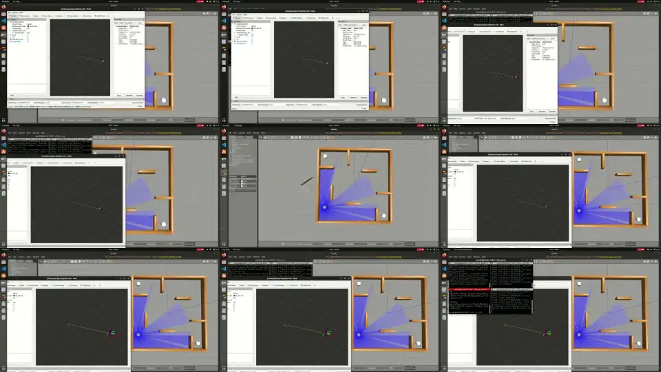*Figure 1 — Sampled rollouts (grey) and the selected trajectory (bright). Extracted frame: frame_002.jpeg.*

Motivation

The goal was to build a readable, tuneable DWA planner that integrates with standard ROS 2 stacks while keeping the rollout and cost logic explicit for easy experimentation. This is useful for coursework and for quickly testing changes to sampling, cost terms, or obstacle handling without diving into larger navigation stacks.

Key ideas and workflow

• Service-driven goal interface: a simple ROS 2 service (togoal) accepts a 2D goal (x, y) and drives the robot toward it. The service node (nav_goal_dwa) repeatedly queries the DWA planner for the best command, publishes visualization markers for rollouts, and sends cmd_vel until the robot is close enough to the goal.
• Planner core: DWAPlannerCustom performs the main work. It:
  • computes the dynamic window from current velocity and acceleration limits,
  • samples linear velocity v and angular velocity w using configured resolutions (v_res_, w_res_),
  • forward-simulates each (v, w) pair over a short horizon (del_T, step dt_) to produce a trajectory,
  • evaluates trajectories using a weighted cost: heading (distance to goal), obstacle proximity, and a velocity term that prefers higher forward speed,
  • returns the best (v, w) and the set of sampled trajectories for visualization.

Algorithmic details

1. Dynamic window: the planner constrains v and w using current velocities curr_vx_, curr_w_ and acceleration bounds acc_v, acc_w, clipped to configured v_min_..v_max_ and w_min_..w_max_.
2. Sampling: linear velocity increments are v_res_ (e.g. 0.08 m/s) and angular increments are w_res_ (e.g. 0.2 rad/s). These control exploration density vs compute cost.
3. Rollouts: each (v, w) pair is simulated for del_T (default 2 s) with integration step dt_ (default 0.05 s). The planner records the sequence of (x, y) points for each rollout.
4. Cost function: the implementation uses three terms with tunable weights (ALPHA, BETA, GAMMA):
   • Heading cost: Euclidean distance from rollout endpoint to goal (encourages progress toward target).
   • Obstacle cost: aggregated penalty where trajectory points fall within an inflation_rad of known obstacles (derived from LaserScan transformed into global obstacle points).
   • Velocity cost: a small cost that biases selection toward higher forward velocities (favors faster trajectories when safe).

The planner selects the rollout with minimum total cost and publishes the corresponding command.

Pseudocode (concise)

loop:
	read odom, scan
	compute dynamic_window from curr_v, curr_w, acc limits
	for v in linspace(min_v, max_v, v_res):
		for w in linspace(min_w, max_w, w_res):
			traj = simulate(v, w, dt, del_T)
			if any point of traj too close to obstacle: obstacle_cost += penalty
			heading_cost = distance(traj.end, goal)
			velocity_cost = v_max - v
			total = ALPHA*heading_cost + BETA*obstacle_cost + GAMMA*velocity_cost
			remember traj and total
	choose traj with min total
	publish cmd_vel for its (v, w)
	publish markers for visualization
	stop when distance(goal, last_point) < threshold

Why these choices

• Sampling resolution (v_res_, w_res_) trades CPU for pathway quality. For TurtleBot3 I used relatively coarse angular steps (0.2 rad/s) and tighter linear steps (0.08 m/s) because small forward-speed changes matter more for steady progress in narrow corridors.
• Rollout horizon (del_T) of 2 s with dt=0.05 s gives enough lookahead to avoid near obstacles while keeping per-cycle simulation count manageable.
• The obstacle penalty multiplies how close a trajectory point is to an obstacle by an inflation constant — this is a simple, robust local safety cue that behaved well with noisy LiDAR in simulation.

Visualization and validation

I publish every sampled rollout as a visualization_msgs::msg::MarkerArray and draw the best trajectory thicker and brighter. This visual feedback is invaluable for tuning: you can change a weight and immediately see how the planner’s preferences shift.

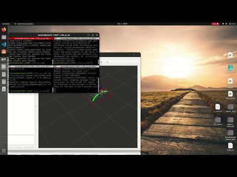
*Figure 2 — Candidate rollouts demonstrating obstacle avoidance and trajectory pruning. Frame from demo video (approx. 00:20–00:30).* 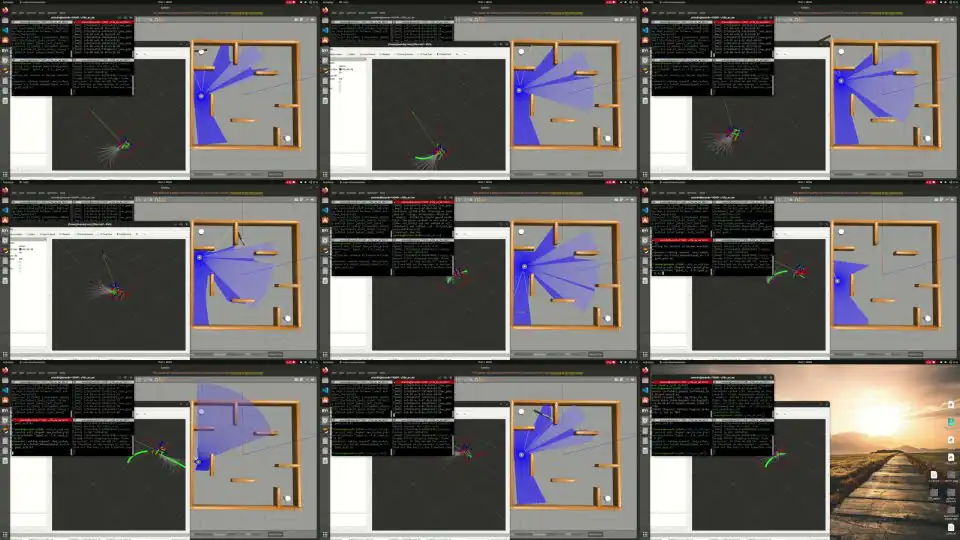*Figure 2 — Candidate rollouts demonstrating obstacle avoidance and trajectory pruning. Extracted frame: frame_006.jpeg.*

If you want higher quality stills from the video for the post, extract frames locally with youtube-dl / yt-dlp and ffmpeg:

yt-dlp -f bestvideo https://youtu.be/y8iu5mr0jKo -o demo.mp4
ffmpeg -ss 00:00:10 -i demo.mp4 -frames:v 1 frame_10.jpg

Below is an additional frame taken from the storyboard extraction that highlights a close-obstacle scenario used to tune the inflation_rad parameter:

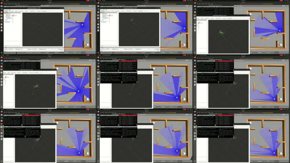*Figure 3 — Close-obstacle rollback case used during parameter tuning. Extracted frame: frame_010.jpeg.`

## ROS 2 integration and differences from common navigation workflows

- The project deliberately avoids a full `nav2` integration and implements a focused local planner instead. This keeps the control loop transparent for tuning and learning.
- The goal interface is a short-lived service that spawns a `DWAPlannerCustom` instance and runs an iterative control loop until the goal is reached. The repository notes that converting the service to an action server would be a robust next step (actions provide feedback and preemption semantics better suited for long-running moves).
- The planner uses `rclcpp::spin_some(dwa)` inside the service loop to let subscriptions (odom, scan) update the planner state. This is a simple approach for the assignment, but in production an action-based loop or keeping the planner node alive and communicating with it via topics/services is preferable.

## Implementation notes and practical tips

- Obstacle mapping: `scanCallback` converts `LaserScan` ranges into global (x, y) points using the current pose and yaw. The planner stores obstacles as a vector of coordinate pairs used to compute `obstacle_cost` for each point on a rollout.
- Parameter tuning: weights (ALPHA, BETA, GAMMA), `inflation_rad`, sampling resolutions, and `del_T`/`dt_` are exposed as constants in the planner header. Moving these parameters to a `params.yaml` (as suggested in the README) makes tuning cleaner and avoids recompiles.
- Visualization: `nav_goal_dwa` publishes a `visualization_msgs::msg::MarkerArray` for all sampled rollouts and highlights the chosen trajectory. This is helpful when tuning because you can see the candidate motions in `rviz2` while changing parameters.
- Safety: the planner stops by publishing zero velocities once the target is reached or on exit. The README suggests adding IMU-based flip detection and handling the goal-inside-obstacle case more gracefully.

## How to run

Follow the repository instructions (condensed):

1. Create a workspace and clone the repo into `src`.
2. Install dependencies and `colcon build` the workspace.
3. Launch the TurtleBot3 Gazebo world and run the `nav_goal_dwa` node:

```bash
source ~/10x_av_ws/install/setup.bash
ros2 run dwa_custom_planner nav_goal_dwa

1. Call the togoal service with goal coordinates (example):

ros2 service call /togoal dwa_custom_planner/srv/ToGoal "{goal_x: 1.2, goal_y: 2.0}"

1. Open rviz2 with the included config to observe rollouts and the selected trajectory.

---

If you’d like, I can:

• add a params.yaml and replace the hard-coded constants with ROS 2 parameters (recommended),
• convert the togoal service into an action server so you get feedback and preemption,
• extract a small set of annotated frames from the demo video and add them into assets/images so the post contains local images instead of external links.

Tell me which next step you want and I’ll implement it.

Lessons and next steps

• Move parameters to a YAML file and load them via ROS 2 parameter APIs for live tuning.
• Convert the service into an action server to support preemption and richer feedback.
• Improve obstacle handling: skip goals inside obstacles, incorporate dynamic obstacle prediction, and add a fail-safe when no safe rollout exists.
• Consider reducing compute by using an early-exit heuristic for rollouts that quickly violate safety (e.g., stop rollout simulation once a point falls inside inflation radius).

References

• Github
• Example video demo linked in the repository README.

If you want, I can convert the hard-coded parameters into a params.yaml and wire them into DWAPlannerCustom for runtime tuning. I can also change the togoal service into an action server in a follow-up commit.